class: center, middle, inverse, title-slide # Multiple Logistic Regression --- layout: true <div class="my-footer"> <span> by Dr. Lucy D'Agostino McGowan </span> </div> --- --- ## Types of statistical models response | predictor(s) | model ---------|--------------|------ quantitative | one quantitative | simple linear regression quantitative | two or more (of either kind) | multiple linear regression binary | one (of either kind) | simple logistic regression binary | two or more (of either kind) | multiple logistic regression --- ## Types of statistical models response | predictor(s) | model ---------|--------------|------ quantitative | one quantitative | simple linear regression quantitative | two or more (of either kind) | multiple linear regression binary | one (of either kind) | simple logistic regression **binary** | **two or more (of either kind)** | **multiple logistic regression** --- ## Types of statistical models variables | predictor | ordinary regression | logistic regression ---|---|---|--- one: `\(x\)` | `\(\beta_0 + \beta_1 x\)` | Response `\(y\)` | `\(\textrm{logit}(\pi)=\log\left(\frac{\pi}{1-\pi}\right)\)` several: `\(x_1,x_2,\dots,x_k\)`| `\(\beta_0 + \beta_1x_1 + \dots+\beta_kx_k\)`|Response `\(y\)` | `\(\textrm{logit}(\pi)=\log\left(\frac{\pi}{1-\pi}\right)\)` --- ## Multiple logistic regression * ✌️ forms Form | Model -----|------ Logit form | `\(\log\left(\frac{\pi}{1-\pi}\right) = \beta_0 + \beta_1x_1 + \beta_2x_2 + \dots \beta_kx_k\)` Probability form | `\(\Large\pi = \frac{e^{\beta_0 + \beta_1x_1 + \beta_2x_2 + \dots \beta_kx_k}}{1+e^{\beta_0 + \beta_1x_1 + \beta_2x_2 + \dots \beta_kx_k}}\)` --- # Steps for modeling 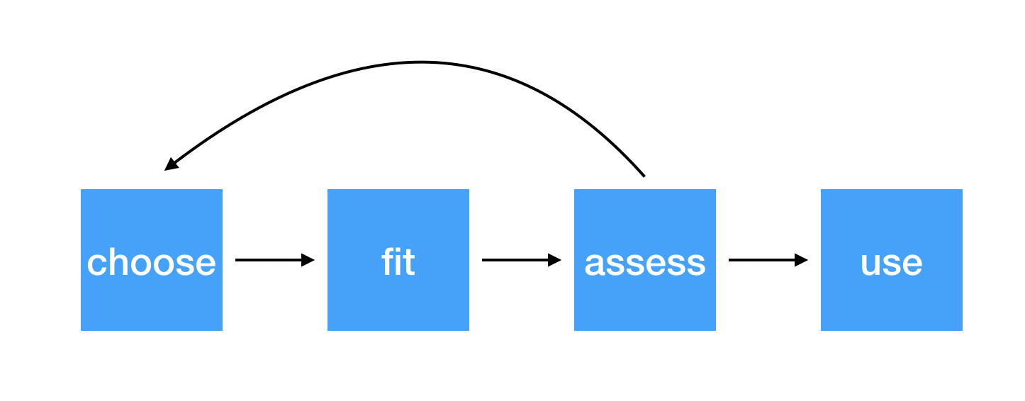 --- ## Fit .small[ ```r data(MedGPA) glm(Acceptance ~ MCAT + GPA, data = MedGPA, family = "binomial") %>% tidy(conf.int = TRUE) ``` ``` ## # A tibble: 3 x 7 ## term estimate std.error statistic p.value conf.low conf.high ## <chr> <dbl> <dbl> <dbl> <dbl> <dbl> <dbl> ## 1 (Intercept) -22.4 6.45 -3.47 0.000527 -36.9 -11.2 ## 2 MCAT 0.165 0.103 1.59 0.111 -0.0260 0.383 ## 3 GPA 4.68 1.64 2.85 0.00439 1.74 8.27 ``` ] --- ## Fit .question[ What does this do? ] .small[ ```r *glm(Acceptance ~ MCAT + GPA, data = MedGPA, family = "binomial") %>% tidy(conf.int = TRUE) ``` ``` ## # A tibble: 3 x 7 ## term estimate std.error statistic p.value conf.low conf.high ## <chr> <dbl> <dbl> <dbl> <dbl> <dbl> <dbl> ## 1 (Intercept) -22.4 6.45 -3.47 0.000527 -36.9 -11.2 ## 2 MCAT 0.165 0.103 1.59 0.111 -0.0260 0.383 ## 3 GPA 4.68 1.64 2.85 0.00439 1.74 8.27 ``` ] --- ## Fit .question[ What does this do? ] .small[ ```r glm(Acceptance ~ MCAT + GPA, data = MedGPA, family = "binomial") %>% * tidy(conf.int = TRUE) ``` ``` ## # A tibble: 3 x 7 ## term estimate std.error statistic p.value conf.low conf.high ## <chr> <dbl> <dbl> <dbl> <dbl> <dbl> <dbl> ## 1 (Intercept) -22.4 6.45 -3.47 0.000527 -36.9 -11.2 ## 2 MCAT 0.165 0.103 1.59 0.111 -0.0260 0.383 ## 3 GPA 4.68 1.64 2.85 0.00439 1.74 8.27 ``` ] --- ## Fit .question[ What does this do? ] .small[ ```r glm(Acceptance ~ MCAT + GPA, data = MedGPA, family = "binomial") %>% tidy(conf.int = TRUE) %>% * kable() ``` ] .small[ <table> <thead> <tr> <th style="text-align:left;"> term </th> <th style="text-align:right;"> estimate </th> <th style="text-align:right;"> std.error </th> <th style="text-align:right;"> statistic </th> <th style="text-align:right;"> p.value </th> <th style="text-align:right;"> conf.low </th> <th style="text-align:right;"> conf.high </th> </tr> </thead> <tbody> <tr> <td style="text-align:left;"> (Intercept) </td> <td style="text-align:right;"> -22.373 </td> <td style="text-align:right;"> 6.454 </td> <td style="text-align:right;"> -3.47 </td> <td style="text-align:right;"> 0.001 </td> <td style="text-align:right;"> -36.894 </td> <td style="text-align:right;"> -11.235 </td> </tr> <tr> <td style="text-align:left;"> MCAT </td> <td style="text-align:right;"> 0.165 </td> <td style="text-align:right;"> 0.103 </td> <td style="text-align:right;"> 1.59 </td> <td style="text-align:right;"> 0.111 </td> <td style="text-align:right;"> -0.026 </td> <td style="text-align:right;"> 0.383 </td> </tr> <tr> <td style="text-align:left;"> GPA </td> <td style="text-align:right;"> 4.676 </td> <td style="text-align:right;"> 1.642 </td> <td style="text-align:right;"> 2.85 </td> <td style="text-align:right;"> 0.004 </td> <td style="text-align:right;"> 1.739 </td> <td style="text-align:right;"> 8.272 </td> </tr> </tbody> </table> ] --- ## Assess .question[ What are the assumptions of multiple logistic regression? ] -- * Linearity * Independence * Randomness --- ## Assess .question[ How do you determine whether the conditions are met? ] * Linearity * Independence * Randomness --- ## Assess .question[ How do you determine whether the conditions are met? ] * Linearity: empirical logit plots * Independence: look at the data generation process * Randomness: look at the data generation process (does the spinner model make sense?) --- ## Assess .question[ If I have two nested models, how do you think I can determine if the full model is significantly better than the reduced? ] -- * We can compare values of `\(-2 \log(\mathcal{L})\)` (deviance) between the two models -- * Calculate the "drop in deviance" the difference between `\((-2 \log(\mathcal{L}_{reduced})) - ( -2 \log(\mathcal{L}_{full}))\)` -- * This is a "likelihood ratio test" -- * This is `\(\chi^2\)` distributed with `\(p\)` degrees of freedom -- * `\(p\)` is the difference in number of predictors between the full and reduced models --- ## Assess * We want to compare a model with GPA and MCAT to one with only GPA .small[ ```r glm(Acceptance ~ GPA, data = MedGPA, family = binomial) %>% glance() ``` ``` ## # A tibble: 1 x 7 ## null.deviance df.null logLik AIC BIC deviance df.residual ## <dbl> <int> <dbl> <dbl> <dbl> <dbl> <int> ## 1 75.8 54 -28.4 60.8 64.9 56.8 53 ``` ] .small[ ```r glm(Acceptance ~ GPA + MCAT, data = MedGPA, family = binomial) %>% glance() ``` ``` ## # A tibble: 1 x 7 ## null.deviance df.null logLik AIC BIC deviance df.residual ## <dbl> <int> <dbl> <dbl> <dbl> <dbl> <int> ## 1 75.8 54 -27.0 60.0 66.0 54.0 52 ``` ] .small[ ```r 56.83901 - 54.01419 ``` ``` ## [1] 2.82 ``` ] --- ## Assess * We want to compare a model with GPA and MCAT to one with only GPA .small[ ```r glm(Acceptance ~ GPA, data = MedGPA, family = binomial) %>% glance() ``` ``` ## # A tibble: 1 x 7 ## null.deviance df.null logLik AIC BIC deviance df.residual ## <dbl> <int> <dbl> <dbl> <dbl> <dbl> <int> ## 1 75.8 54 -28.4 60.8 64.9 56.8 53 ``` ] .small[ ```r glm(Acceptance ~ GPA + MCAT, data = MedGPA, family = binomial) %>% glance() ``` ``` ## # A tibble: 1 x 7 ## null.deviance df.null logLik AIC BIC deviance df.residual ## <dbl> <int> <dbl> <dbl> <dbl> <dbl> <int> ## 1 75.8 54 -27.0 60.0 66.0 54.0 52 ``` ] .small[ ```r pchisq(56.83901 - 54.01419 , df = 1, lower.tail = FALSE) ``` ``` ## [1] 0.0928 ``` ] --- ## Assess * We want to compare a model with GPA, MCAT, and number of applications to one with only GPA .small[ ```r glm(Acceptance ~ GPA, data = MedGPA, family = "binomial") %>% glance() ``` ``` ## # A tibble: 1 x 7 ## null.deviance df.null logLik AIC BIC deviance df.residual ## <dbl> <int> <dbl> <dbl> <dbl> <dbl> <int> ## 1 75.8 54 -28.4 60.8 64.9 56.8 53 ``` ] .small[ ```r glm(Acceptance ~ GPA + MCAT + Apps, data = MedGPA, family = "binomial") %>% glance() ``` ``` ## # A tibble: 1 x 7 ## null.deviance df.null logLik AIC BIC deviance df.residual ## <dbl> <int> <dbl> <dbl> <dbl> <dbl> <int> ## 1 75.8 54 -26.8 61.7 69.7 53.7 51 ``` ] .small[ ```r pchisq(56.83901 - 53.68239, df = 2, lower.tail = FALSE) ``` ``` ## [1] 0.206 ``` ] --- ## Use * We can calculate confidence intervals for the `\(\beta\)` coefficients: `\(\hat\beta\pm z^*\times SE_{\hat\beta}\)` * To determine whether individual explanatory variables are statistically significant, we can calculate p-values based on the `\(z\)`-statistic of the `\(\beta\)` coefficients (using the normal distribution) --- ## Use .question[ How do you interpret these `\(\beta\)` coefficients? ] .small[ ```r glm(Acceptance ~ MCAT + GPA, data = MedGPA, family = "binomial") %>% tidy(conf.int = TRUE) ``` ``` ## # A tibble: 3 x 7 ## term estimate std.error statistic p.value conf.low conf.high ## <chr> <dbl> <dbl> <dbl> <dbl> <dbl> <dbl> ## 1 (Intercept) -22.4 6.45 -3.47 0.000527 -36.9 -11.2 ## 2 MCAT 0.165 0.103 1.59 0.111 -0.0260 0.383 ## 3 GPA 4.68 1.64 2.85 0.00439 1.74 8.27 ``` ] --- class: middle ## `\(\hat\beta\)` interpretation in multiple logistic regression The coefficient for `\(x\)` is `\(\hat\beta\)` (95% CI: `\(LB_\hat\beta, UB_\hat\beta\)`). A one-unit increase in `\(x\)` yields a `\(\hat\beta\)` expected change in the log odds of y, **holding all other variables constant**. --- class: middle ## `\(e^{\hat\beta}\)` interpretation in multiple logistic regression The odds ratio for `\(x\)` is `\(e^{\hat\beta}\)` (95% CI: `\(e^{LB_\hat\beta}, e^{UB_\hat\beta}\)`). A one-unit increase in `\(x\)` yields a `\(e^{\hat\beta}\)`-fold expected change in the odds of y, **holding all other variables constant**. --- ## Summary | Ordinary regression | Logistic regression ---|------|---- test or interval for `\(\beta\)` | `\(t = \frac{\hat\beta}{SE_{\hat\beta}}\)` | `\(z = \frac{\hat\beta}{SE_{\hat\beta}}\)` | | t-distribution | z-distribution test for nested models | `\(F = \frac{\Delta SSModel / p}{SSE_{full} / (n - k - 1)}\)` | G = `\(\Delta(-2\log\mathcal{L})\)`| | F-distribution | `\(\chi^2\)`-distribution