class: center, middle, inverse, title-slide # Assessing Assumptions: Independence and Randomness --- layout: true <div class="my-footer"> <span> by Dr. Lucy D'Agostino McGowan </span> </div> --- # Steps for modeling 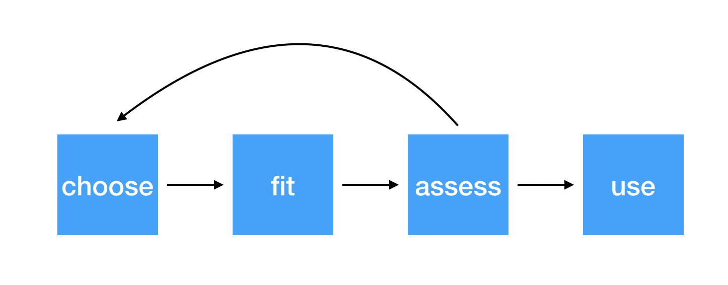 --- ## Conditions for ordinary linear regression * Linearity * Zero Mean * Constant Variance * Independence * Random * Normality --- ## Conditions for ordinary linear regression .small[ Assumption| What it means | How do you check? | How do you fix? ----|-----|-----------|----- Linearity |The relationship between the outcome and explanatory variable or predictor is linear **holding all other variables constant**| Residuals vs. fits plot | fit a better model (transformations, polynomial terms, more / different variables, etc.) Zero Mean | | | ] --- ## Conditions for ordinary linear regression .small[ Assumption| What it means | How do you check? | How do you fix? ----|-----|-----------|----- Linearity |The relationship between the outcome and explanatory variable or predictor is linear **holding all other variables constant**| Residuals vs. fits plot | fit a better model (transformations, polynomial terms, more / different variables, etc.) Zero Mean | The error distribution is centered at zero | by default | -- Constant Variance | | | ] --- ## Conditions for ordinary linear regression .small[ Assumption| What it means | How do you check? | How do you fix? ----|-----|-----------|----- Linearity |The relationship between the outcome and explanatory variable or predictor is linear **holding all other variables constant**| Residuals vs. fits plot | fit a better model (transformations, polynomial terms, more / different variables, etc.) Zero Mean | The error distribution is centered at zero | by default | -- Constant Variance | The variability in the errors is the same for all values of the predictor variable | Residuals vs fits plot | fit a better model Independence | | | ] --- ## Conditions for ordinary linear regression .small[ Assumption| What it means | How do you check? | How do you fix? ----|-----|-----------|----- Linearity |The relationship between the outcome and explanatory variable or predictor is linear **holding all other variables constant**| Residuals vs. fits plot | fit a better model (transformations, polynomial terms, more / different variables, etc.) Zero Mean | The error distribution is centered at zero | by default | -- Constant Variance | The variability in the errors is the same for all values of the predictor variable | Residuals vs fits plot | fit a better model Independence | The errors are assumed to be independent from one another | 👀 data generation | Find better data or fit a fancier model Random | | | ] --- ## Conditions for ordinary linear regression .small[ Assumption| What it means | How do you check? | How do you fix? ----|-----|-----------|----- Linearity |The relationship between the outcome and explanatory variable or predictor is linear **holding all other variables constant**| Residuals vs. fits plot | fit a better model (transformations, polynomial terms, more / different variables, etc.) Zero Mean | The error distribution is centered at zero | by default | -- Constant Variance | The variability in the errors is the same for all values of the predictor variable | Residuals vs fits plot | fit a better model Independence | The errors are assumed to be independent from one another | 👀 data generation | Find better data or fit a fancier model Random | The data are obtained using a random process | 👀 data generation | Find better data or fit a fancier model Normality | | | ] --- ## Conditions for ordinary linear regression .small[ Assumption| What it means | How do you check? | How do you fix? ----|-----|-----------|----- Linearity |The relationship between the outcome and explanatory variable or predictor is linear **holding all other variables constant**| Residuals vs. fits plot | fit a better model (transformations, polynomial terms, more / different variables, etc.) Zero Mean | The error distribution is centered at zero | by default | -- Constant Variance | The variability in the errors is the same for all values of the predictor variable | Residuals vs fits plot | fit a better model Independence | The errors are assumed to be independent from one another | 👀 data generation | Find better data or fit a fancier model Random | The data are obtained using a random process | 👀 data generation | Find better data or fit a fancier model Normality | The random errors follow a normal distribution | QQ-plot / residual histogram | fit a better model ] --- ## Conditions for **logistic** regression * Linearity * Independence * Randomness --- ## Conditions for **logistic** regression .question[ How do we test linearity? ] * **Linearity** * Independence * Randomness --- ## Conditions for **logistic** regression .question[ How do we test linearity? ] * **Linearity** ✅ _Plot the empirical logits_ * Independence * Randomness --- ## ⛳ Testing for linearity in logistic regression * We can plot the **empirical logit** to examine the linearity assumption Length | 3 | 4 | 5 | 6 | 7 ------|----|---|---|---|--- Number of successes | 84 | 88 | 61 | 61 | 44 Number of failures | 17 | 31 | 47 | 64 | 90 Total | 101 | 119 | 108 | 125 | 134 Probability of success | 0.832 | 0.739 | 0.565 | 0.488 | 0.328 Odds of success | 4.941 | 2.839 | 1.298| 0.953| 0.489 Empirical logit | 1.60 | 1.04| 0.26 |−0.05 |−0.72 --- ## ⛳ Testing for linearity in logistic regression .small[ ```r data <- data.frame( length = c(3, 4, 5, 6, 7), emp_logit = c(1.6, 1.04, 0.26, -0.05, -0.72) ) ggplot(data, aes(length, emp_logit)) + geom_point() + geom_abline(intercept = 3.26, slope = -0.566, lty = 2) + labs(y = "log odds of success") ``` 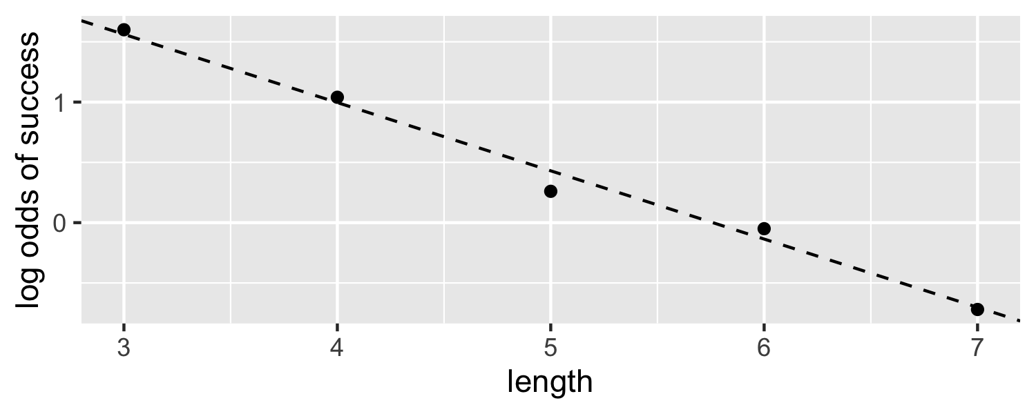<!-- --> ] --- # Conditions for **logistic** regression * Linearity * **Independence** * **Randomness** --- ## Why do we care? 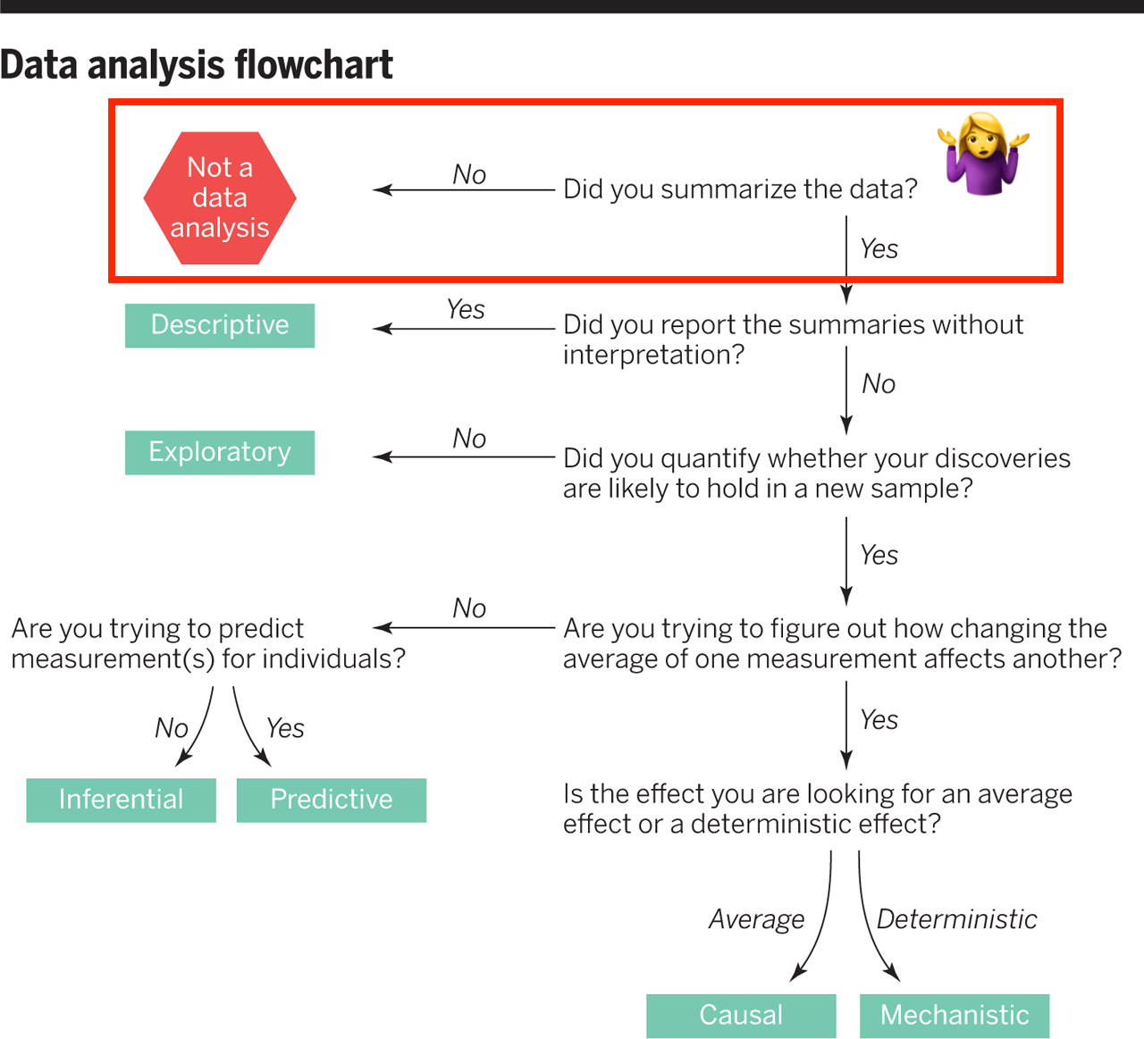 --- ## Why do we care? 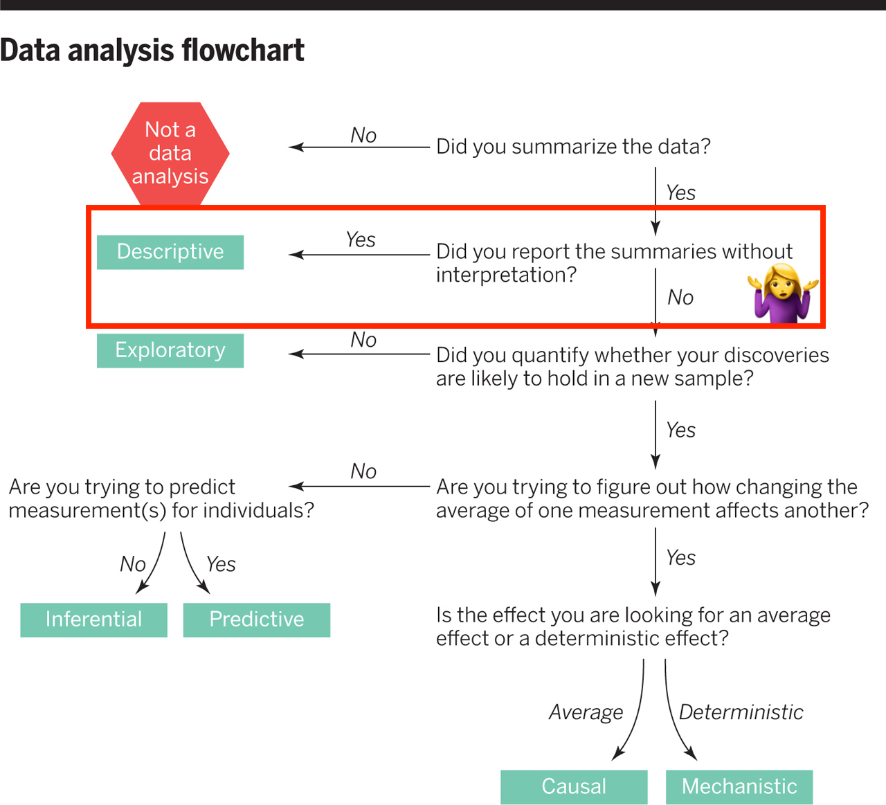 --- ## Why do we care?  --- ## Why do we care?  --- ## Independence * The observations should be _independent_ of one another * In the Medical School Admission - GPA example, 55 students were randomly selected and their admission status and GPA were recorded: 👍 Independent or 👎 Not? -- * 👍 -- * A new treatment comes out to help with dry eyes. A sample of 25 people get randomized to either treatment or placebo - this creates a dataset of information about 50 eyes. 👍 or 👎 -- * 👎 --- ## Randomness .question[ What do I put for the **family** argument if I want to fit a logistic regression in R? ] ```r glm(am ~ mpg, data = mtcars, * family = "---") ``` --- ## Randomness .question[ What do I put for the **family** argument if I want to fit a logistic regression in R? ] ```r glm(am ~ mpg, data = mtcars, * family = "binomial") ``` * The **binomial** distribution tells you the number of successes in `\(n\)` experiments -- * For the purposes of this class, `\(n\)` will always be 1 -- * This is special case of the **binomial** distribution, called the **Bernoulli** distribution -- * Why does this matter? R wants you to specify that you are using the `"binomial"` family, your book talks about the **Bernoulli** distribution, I just want to bridge the gap --- ## Randomness _The Spinner_ * A random 0, 1 outcome that behaves like a "spinner" follows the **Bernoulli** distribution -- * For example, in a fair coin toss, the probability of getting "heads" is 50% <!-- --> --- ## Randomness _The Spinner_ * A random 0, 1 outcome that behaves like a "spinner" follows the **Bernoulli** distribution * For example, in a fair coin toss, the probability of getting "heads" is 50% <!-- --> --- ## Randomness _The Spinner_ * A random 0, 1 outcome that behaves like a "spinner" follows the **Bernoulli** distribution * For example, in a fair coin toss, the probability of getting "heads" is 50% <!-- --> --- ## Randomness _The Spinner_ * A random 0, 1 outcome that behaves like a "spinner" follows the **Bernoulli** distribution * For example, in a fair coin toss, the probability of getting "heads" is 50% <!-- --> --- ## Randomness _The Spinner_ * A random 0, 1 outcome that behaves like a "spinner" follows the **Bernoulli** distribution * In the Medical school admissions - GPA example, a student with a 3.8 has an 82% chance of acceptance <!-- --> --- ## Randomness _The Spinner_ * A random 0, 1 outcome that behaves like a "spinner" follows the **Bernoulli** distribution * In the Medical school admissions - GPA example, a student with a 3.8 has an 82% chance of acceptance <!-- --> --- ## Randomness _The Spinner_ * A random 0, 1 outcome that behaves like a "spinner" follows the **Bernoulli** distribution * In the Medical school admissions - GPA example, a student with a 3.8 has an 82% chance of acceptance <!-- --> --- ## Randomness _The Spinner_ * A random 0, 1 outcome that behaves like a "spinner" follows the **Bernoulli** distribution * In the Medical school admissions - GPA example, a student with a 3.8 has an 82% chance of acceptance <!-- --> --- ## Randomness _The Spinner_ * A random 0, 1 outcome that behaves like a "spinner" follows the **Bernoulli** distribution * In the Medical school admissions - GPA example, a student with a 3.8 has an 82% chance of acceptance <!-- -->