Variable Transformations Recap

# Variable Transformations Recap

---

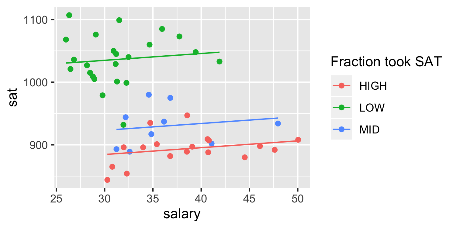
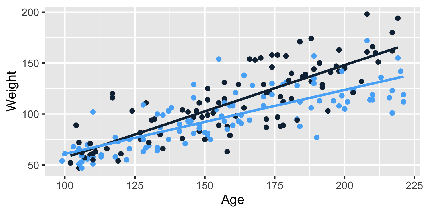
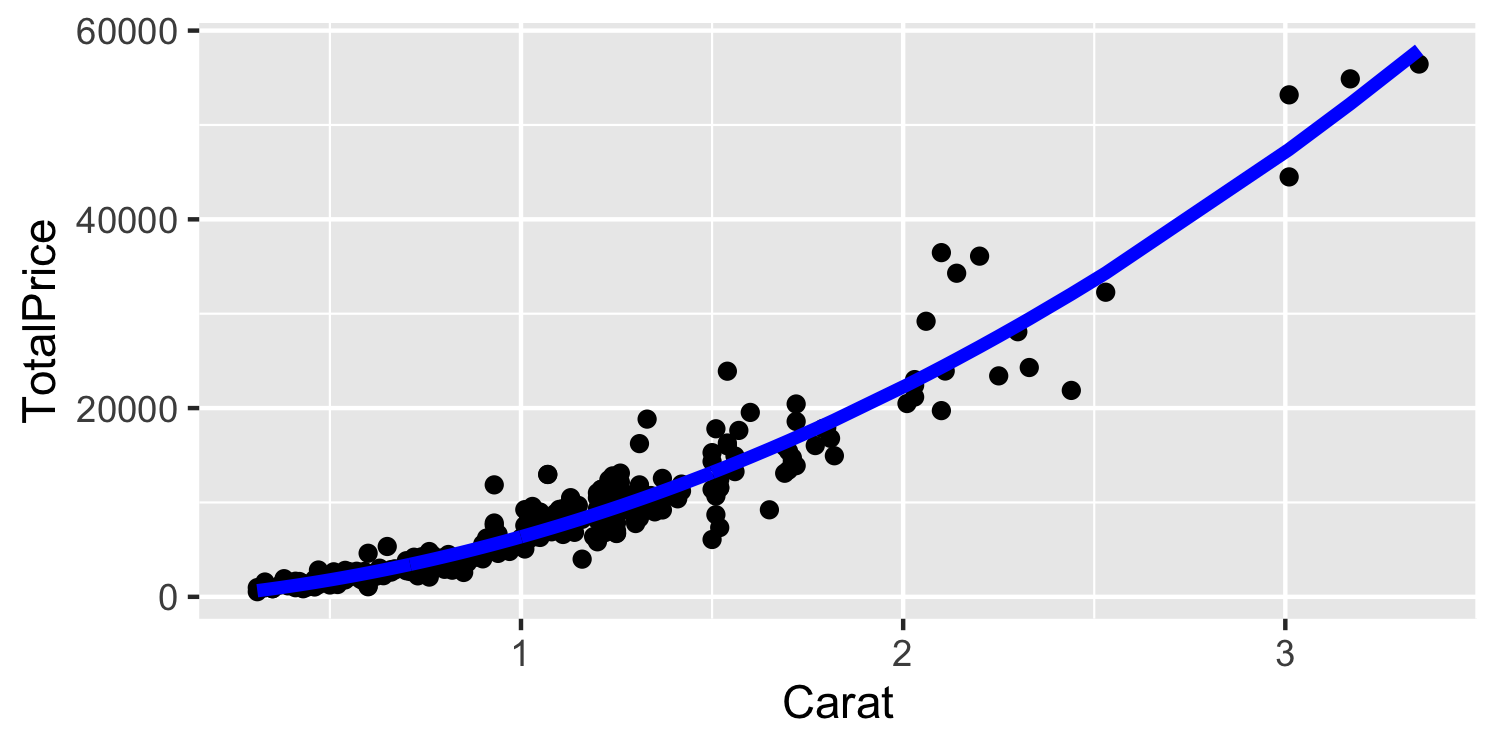
<div class="my-footer">
<span>
by Dr. Lucy D'Agostino McGowan
</span>
</div>

---

## `\(\hat\beta\)` interpretation in multiple linear regression

The coefficient for `\(x\)` is `\(\hat\beta\)` (95% CI: `\(LB_\hat\beta, UB_\hat\beta\)`). A one-unit increase in `\(x\)` yields an expected increase in y of `\(\hat\beta\)`, **holding all other variables constant**.

---

## `\(\hat\beta_1\)` interpretation in

`\(sat = \beta_0 + \beta_1salary + \beta_2 (frac = LOW) + \beta_3 (frac = HIGH) + \epsilon\)`

The coefficient for average salary is 1.09 (95% CI: -0.90, 3.08).  A one-unit increase in average salary yields an expected increase in average SAT score of 1.09, **holding the fraction of students that took the SAT constant**.

---

## Adjusting for confoundrs

![](10-variable-transformations-recap_files/figure-html/unnamed-chunk-2-1.png)

* The lines are **parallel**, the slope ( `\(\hat\beta_1\)` ) is **constant** between groups

---

## Interactions

![](10-variable-transformations-recap_files/figure-html/unnamed-chunk-3-1.png)

* 😱 the lines cross! That means there is an **interaction**, that is the slopes differ based on the group

---

## Interactions

`\(Weight = \beta_0 + \beta_1 Age + \beta_2 Girl + \beta_3 Age \times Girl + \epsilon\)`

```r
lm(Weight ~ Age + Sex + Age * Sex, data = Kids198)
```

```
## 
## Call:
## lm(formula = Weight ~ Age + Sex + Age * Sex, data = Kids198)
## 
## Coefficients:
## (Intercept)          Age          Sex      Age:Sex  
##    -33.6925       0.9087      31.8506      -0.2812
```
]

* What does this model become for **boys** (When `Sex = 0`)

--
  * `\(Weight = \beta_0 + \beta_1 Age + \epsilon\)`

--
* What does this model become for **girls** (When `Sex = 1`)

--
  * `\(Weight = \beta_0 + \beta_1 Age + \beta_2 1 + \beta_3 Age \times 1 + \epsilon\)`

--
  * `\(Weight = (\beta_0 + \beta_2) + (\beta_1 + \beta_3) Age  + \epsilon\)`

--
* How do you interpret `\(\hat\beta_0\)` now?

---

## Interactions

```r
lm(Weight ~ Age + Sex + Age * Sex, data = Kids198)
```

* What does this model become for **boys** (When `Sex = 0`)
  * `\(Weight = \beta_0 + \beta_1 Age + \epsilon\)`
* What does this model become for **girls** (When `Sex = 1`)
  * `\(Weight = \beta_0 + \beta_1 Age + \beta_2 1 + \beta_3 Age \times 1 + \epsilon\)`
  * `\(Weight = (\beta_0 + \beta_2) + (\beta_1 + \beta_3) Age  + \epsilon\)`
* How do you interpret `\(\hat\beta_{2}\)` now?

--
  * The difference in intercepts between boys and girls

---

## Interactions

```r
lm(Weight ~ Age + Sex + Age * Sex, data = Kids198)
```

--
  * How much the slope changes as we move from the regression line for boys to that for girls

---

## `\(\hat\beta\)` interpretation for interactions between `\(x\)` and a binary indicator `\(I\)`

The coefficient for the interaction between `\(x\)` and `\(I\)` is `\(\hat\beta\)` (95% CI: `\(LB_\hat\beta, UB_\hat\beta\)`). This means that the effect of `\(x\)` on `\(y\)` differs by `\(\hat\beta\)` when `\(I = 1\)` compared to `\(I = 0\)` **holding all other variables constant***.

--
* You must include this line if there are **additional variables in your model**.

---

## `\(\hat\beta_3\)` interpretation for

`\(Weight = \beta_0 + \beta_1 Age + \beta_2 Girl + \beta_3 Age \times Girl + \epsilon\)`

The coefficient for the interaction between `Age` and `Sex` is -0.28 (95% CI: -0.44, -0.12). This means that the effect of `Age` on `Weight` lower by 0.28 among girls compared to boys.

---

## Non-linear relationships

```r
lm(TotalPrice ~ Carat + I(Carat^2), data = Diamonds)
```

![](10-variable-transformations-recap_files/figure-html/unnamed-chunk-8-1.png)

* What is the equation for this relationship?

---

## Interpreting `\(\hat\beta\)`s in the presence of polynomials

`\(Total Price = \beta_0 + \beta_1 Carat + \beta_2 Carat^2 + \epsilon\)`

* What is the interpretation of `\(\hat\beta_1\)`?

--
* Typically, in multiple linear regression, the interpretation of `\(\hat\beta_i\)` is:
a one-unit change in `\(x\)` yields an expected change in `\(y\)` of `\(\hat\beta_i\)` **holding all other variables constant**.

--
  * What does it mean to see a change in `Caret` holding `Carat` `\(^2\)` constant?

--
* When you have a polynomial term, you need to **specify the values you are changing between**, since the change is no longer constant across all values of `\(x\)`.

---

## Interpreting `\(\hat\beta\)` in the presence of polynomials
.small[

```r
lm(TotalPrice ~ Carat + I(Carat^2), data = Diamonds) %>%
  tidy()
```

```
## # A tibble: 3 x 5
##   term        estimate std.error statistic  p.value
##   <chr>          <dbl>     <dbl>     <dbl>    <dbl>
## 1 (Intercept)    -523.      466.     -1.12 2.63e- 1
## 2 Carat          2386.      753.      3.17 1.66e- 3
## 3 I(Carat^2)     4498.      263.     17.1  5.09e-48
```
]

What is the expected change in `TotalPrice` for a one-unit change in `Carat`, changing from 0.8 to 1.8?

```r
(-522.7 + 2386 * 1.8 + 4498.2 * 1.8^2) - 
  (-522.7 + 2386 * 0.8 + 4498.2 * 0.8^2)
```

```
## [1] 14081.32
```
]
]

```r
2386 * (1.8 - 0.8) + 
  4498.2 * (1.8^2 - 0.8^2)
```

```
## [1] 14081.32
```
]
]

---

## Interpreting `\(\hat\beta\)` in the presence of polynomials
.small[

```r
lm(TotalPrice ~ Carat + I(Carat^2), data = Diamonds) %>%
  tidy()
```

What is the expected change in `TotalPrice` for a one-unit change in `Carat`, changing from 1.8 to 2.8?

```r
2386 * (2.8 - 1.8) + 4498.2 * (2.8^2 - 1.8^2)
```

```
## [1] 23077.72
```
]

--
* Can we talk about `\(\hat\beta_1\)` and `\(\hat\beta_2\)` in the context of a one-unit change in `Carat`?

---
## Interpreting `\(\hat\beta\)` in the presence of polynomials

* `\(\hat\beta\)` coefficients that are transformations of the same `\(x\)` variable **must** be interpreted together

--
* You must first choose to values of `\(x\)` to change between, and then report the change.

--
* A sensible choice for the two `\(x\)` values can be the 25th% quantile and the 75th% quantile.

---

## General `\(\hat\beta\)` interpretation with quadratic terms

The linear term in the model for `\(x\)` has a coefficient of `\(\hat\beta_1\)` (95% CI: `\((LB_{\hat\beta_1}, UB_{\hat\beta_1})\)`). The quadratic term in the model for `\(x\)` has a coefficient of `\(\hat\beta_2\)` (95% CI: `\((LB_{\hat\beta_2}, UB_{\hat\beta_2})\)`). A change in `\(x\)` from `\(a\)` to `\(b\)` yields an expected change in `\(y\)` of `\(\hat\beta_1 (b - a) + \hat\beta_2 (b^2 - a^2)\)` **holding all other variables constant***.

--
* You must include this line if there are **additional variables in your model**.

---

## Specific `\(\hat\beta\)` interpretation for `\(y = \beta_0 + \beta_1 Carat + \beta_2 Carat^2 + \epsilon\)` model

The linear term in the model for `Carat` has a coefficient of 2386 (95% CI: `\((906, 3866)\)`). The quadratic term in the model for `Carat` has a coefficient of `\(4498\)` (95% CI: `\((3981, 5016)\)`). A change in `Carat` from `\(0.7\)` to `\(1.24\)` yields an expected change in `TotalPrice` of `\(6000.5\)`.

--
* Where did I get 0.7 and 1.24?

---

## Quantiles

```r
Diamonds %>%
  summarise(q1 = quantile(Carat, 0.25),
            q3 = quantile(Carat, 0.75))
```

```
##    q1   q3
## 1 0.7 1.24
```

---

## <i class="fas fa-laptop"></i> `Diamonds`

- Go to RStudio Cloud and open `Diamonds`
- Fit the model  `\(TotalPrice = \beta_0  + \beta_1Carat + \beta_2 Carat^2 + \beta_3 Color+\epsilon\)`
- Find the 0.25 quantile and 0.75 quantile of `Carat`
- What is the interpretation of `\(\hat\beta_1\)`, `\(\hat\beta_2\)`, and `\(\hat\beta_3\)`?