Multiple linear regression

# Multiple linear regression

---

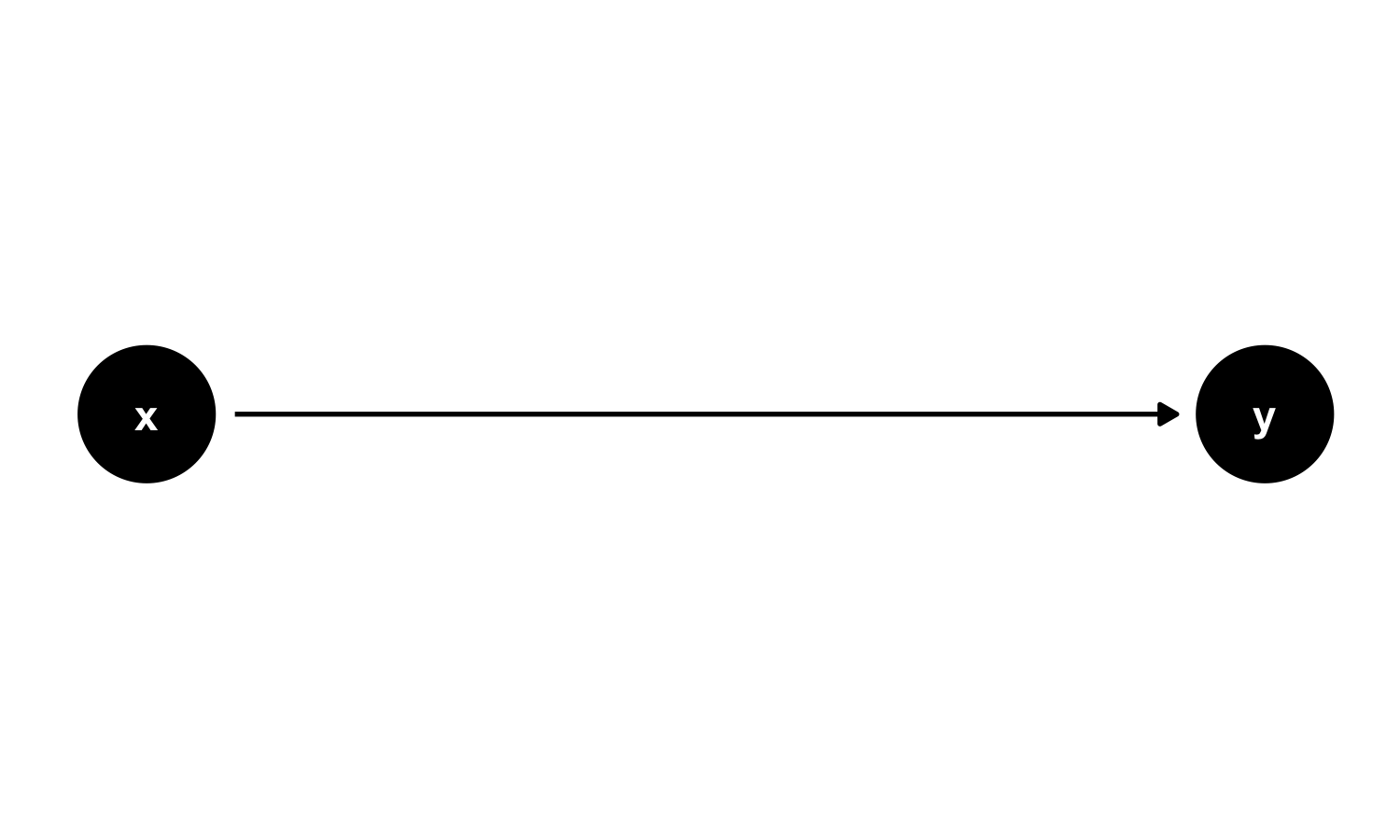
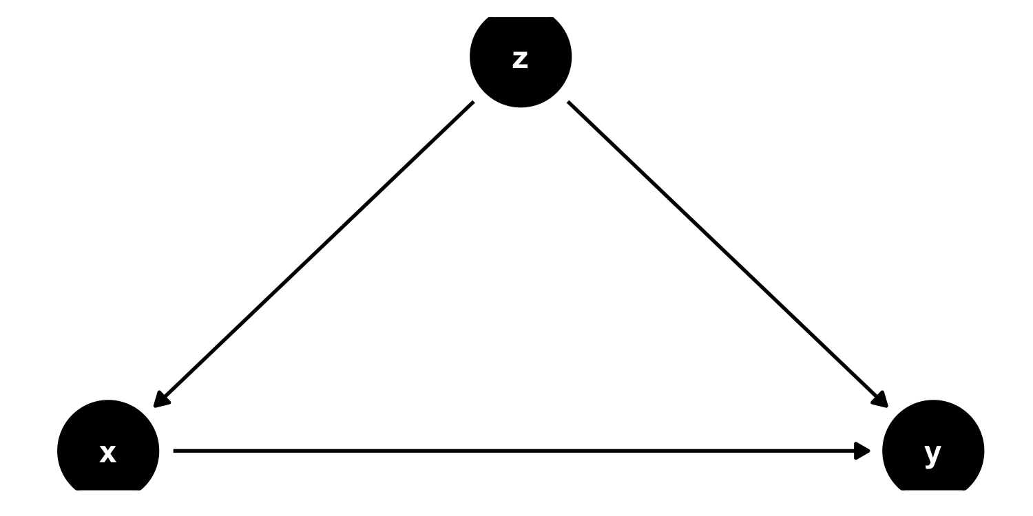
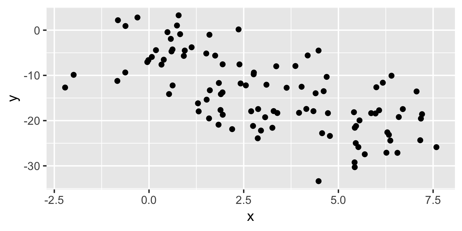
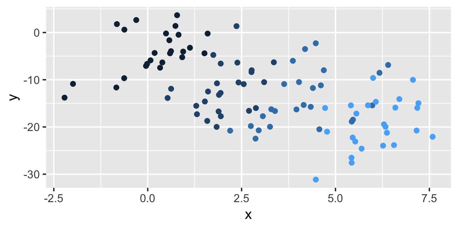
<div class="my-footer">

by Dr. Lucy D'Agostino McGowan

</div>

---

## Simple linear regression

`\(\Huge y = \beta_0 + \beta_1X + \epsilon\)`

`\(\Huge \epsilon\sim N(0,\sigma_\epsilon)\)`
]

---

## Multiple linear regression

.center[
`\(\Large y = \beta_0 + \beta_1X_1 + \beta_2X_2+\dots+\beta_kX_k+ \epsilon\)` 
 
`\(\Huge \epsilon\sim N(0,\sigma_\epsilon)\)`

]

---

## Multiple linear regression

* estimate coefficents that minimize the sum of squared residuals

---

## Let's do it in R!

* Data: Porsche Price
* Price, Mileage, Age

---

## Let's do it in R!

.question[
What is my response variable? What are my explantory variables?
]
* Data: Porsche Price
* Price, Mileage, Age

---

## Let's do it in R!

```r
data("PorschePrice")
lm(Price ~ Mileage + Age, data = PorschePrice)
```

```
## 
## Call:
## lm(formula = Price ~ Mileage + Age, data = PorschePrice)
## 
## Coefficients:
## (Intercept)      Mileage          Age  
##     70.9192      -0.5613      -0.1302
```
]

---

## Let's do it in R!

.question[
What is different between this and the `lm()` functions we have been previously running?
]

```r
data("PorschePrice")
lm(Price ~ Mileage + Age, data = PorschePrice)
```

```
## 
## Call:
## lm(formula = Price ~ Mileage + Age, data = PorschePrice)
## 
## Coefficients:
## (Intercept)      Mileage          Age  
##     70.9192      -0.5613      -0.1302
```
]

---

## Let's do it in R!

.question[
What is different between this and the `lm()` functions we have been previously running?
]

```r
lm(Price ~ Mileage + Age, data = PorschePrice) %>%
  tidy()
```

```
## # A tibble: 3 x 5
## term estimate std.error statistic p.value
## <chr> <dbl> <dbl> <dbl> <dbl>
## 1 (Intercept) 70.9 2.48 28.6 1.04e-21
## 2 Mileage -0.561 0.114 -4.92 3.76e- 5
*## 3 Age -0.130 0.457 -0.285 7.78e- 1
```
]

---

## Let's do it in R!

```r
lm(Price ~ Mileage + Age, data = PorschePrice) %>%
  tidy()
```

---

## Let's do it in R!

```r
lm(Price ~ Mileage + Age, data = PorschePrice) %>%
  predict()
```

```
##        1        2        3        4        5        6        7        8 
## 58.45976 46.39104 59.48812 50.19016 45.69948 42.18328 70.18942 70.54307 
##        9       10       11       12       13       14       15       16 
## 63.13681 65.47420 62.07027 65.32602 59.67674 63.28725 50.58761 54.89194 
##       17       18       19       20       21       22       23       24 
## 58.94700 54.96152 40.59583 52.34120 45.64334 41.27170 50.49105 58.63042 
##       25       26       27       28       29       30 
## 35.07453 41.71625 18.01894 21.23878 20.03975 49.53452
```
]

---

## Let's do it in R!

---

## Let's do it in R!

---

## Let's do it in R!

---

## Let's do it in R!

```r
lm(Price ~ Mileage + Age, data = PorschePrice) %>% 
  anova()
```

```
## Analysis of Variance Table
## 
## Response: Price
##           Df Sum Sq Mean Sq  F value    Pr(>F)
## Mileage    1 5565.7  5565.7 104.7023 8.653e-11
## Age        1    4.3     4.3   0.0813    0.7778
*## Residuals 27 1435.2    53.2
```
]

---
class: center, middle

## Why might we want to do this?

---

http://science.sciencemag.org/content/347/6228/1314

---

## Multiple linear regression for inference

---

## Multiple linear regression for inference

**Goal:** Discover the relationship between a response (outcome, `\(y\)`), and an explanatory variable ( `\(x\)` )

---

## Multiple linear regression for inference

**Goal:** Discover the relationship between a response (outcome, `\(y\)`), and an explanatory variable ( `\(x\)` ) **adjusting for all known confounders**

---

## Multiple linear regression for inference

**Goal:** Discover the relationship between a response (outcome, `\(y\)`), and an explanatory variable ( `\(x\)` ) **adjusting for all known confounders**

---
class: middle

## confounder

A confounder is a variable that is associated with both the response variable ( `\(y\)` ) and the explanatory variable ( `\(x\)` ). If not accounted for, it can result in seeing a spurious relationship between `\(x\)` and `\(y\)`.

---

## Confounder example

![](08-multiple-linear-regression_files/figure-html/unnamed-chunk-8-1.png)

---

## Confounder example

![](08-multiple-linear-regression_files/figure-html/unnamed-chunk-9-1.png)

---

## Confounder example

![](08-multiple-linear-regression_files/figure-html/unnamed-chunk-10-1.png)

---

## Confounder example

![](08-multiple-linear-regression_files/figure-html/unnamed-chunk-11-1.png)

---

## Confounder example

![](08-multiple-linear-regression_files/figure-html/unnamed-chunk-12-1.png)

---

## Confounding example

Armstrong, K.A. (2012). Methods in comparative effectiveness research. _Journal of clinical oncology: official journal of the American Society of Clinical Oncology_, 30 34, 4208-14.
---

## A quick R aside

* So far, the data we've been using has been included in an **R package**
* To access this data we just run `data("data set")`
* What if we want to read in other data, for example from a `.csv` file?
--

* enter: `read_csv()`
--

* `read_csv()` is a function from the **readr** package, which is included when you load the **tidyverse**
--

* it works like this:

```r
df <- read_csv("the-path-to-your-file.csv")
```

Where `df` can be whatever you'd like to call your new dataset
---

## Berkley administration data

* Study carried out by the graduate Division of the University of California, Berkeley in the early 70’s to evaluate whether there was a sex bias in graduate admissions
--

* The data come from six departments. For confidentiality we'll call them A-F.
--

* We have information on whether the applicant was male or female and whether they were admitted or rejected.
--

* First, we will evaluate whether the percentage of males admitted is indeed higher than females, overall. Next, we will calculate the same percentage for each department.

.my-footer[

<img src = "img/dsbox-logo.png" width = "30"> </img> Slides adapted from <a href="https://datasciencebox.org" target="_blank">datasciencebox.org</a> by Dr. Lucy D'Agostino McGowan

]
---

## `UCB admits`

- Go to RStudio Cloud and open `UCB admits`

---

## Berkley admin data

* What was our response variable?
--

* What was our explanatory variable of interest?
--

* What was our confounder?
--

* What was our equation?

---

## Simpson's paradox

![](08-multiple-linear-regression_files/figure-html/unnamed-chunk-14-1.png)

---

## Simpson's paradox

![](08-multiple-linear-regression_files/figure-html/unnamed-chunk-15-1.png)

---

## Porsche data

```r
lm(Price ~ Mileage + Age, data = PorschePrice) %>%
  tidy()
```

```
## # A tibble: 3 x 5
## term estimate std.error statistic p.value
## <chr> <dbl> <dbl> <dbl> <dbl>
## 1 (Intercept) 70.9 2.48 28.6 1.04e-21
## 2 Mileage -0.561 0.114 -4.92 3.76e- 5
## 3 Age -0.130 0.457 -0.285 7.78e- 1
```
]

---

## Porsche data

```r
lm(Price ~ Mileage + Age, data = PorschePrice) %>%
  tidy()
```

```
## # A tibble: 3 x 5
## term estimate std.error statistic p.value
## <chr> <dbl> <dbl> <dbl> <dbl>
## 1 (Intercept) 70.9 2.48 28.6 1.04e-21
## 2 Mileage -0.561 0.114 -4.92 3.76e- 5
## 3 Age -0.130 0.457 -0.285 7.78e- 1
```
]

---

## Porsche data

```r
lm(Price ~ Mileage + Age, data = PorschePrice) %>%
  tidy()
```

```
## # A tibble: 3 x 5
## term estimate std.error statistic p.value
## <chr> <dbl> <dbl> <dbl> <dbl>
## 1 (Intercept) 70.9 2.48 28.6 1.04e-21
## 2 Mileage -0.561 0.114 -4.92 3.76e- 5
## 3 Age -0.130 0.457 -0.285 7.78e- 1
```
]

* `\(\Large t = \frac{\hat\beta_2}{SE_{\hat\beta_2}}\)`
--

* `\(\Large t = \frac{\hat\beta_i}{SE_{\hat\beta_i}}\)`
---

## Porsche data

```r
lm(Price ~ Mileage + Age, data = PorschePrice) %>%
  tidy()
```

```
## # A tibble: 3 x 5
## term estimate std.error statistic p.value
## <chr> <dbl> <dbl> <dbl> <dbl>
## 1 (Intercept) 70.9 2.48 28.6 1.04e-21
## 2 Mileage -0.561 0.114 -4.92 3.76e- 5
## 3 Age -0.130 0.457 -0.285 7.78e- 1
```
]

* `\(\Large H_0: \beta_i = 0\)`
* `\(\Large H_A: \beta_i \neq 0\)`

---

## Porsche data

.question[
What would the degrees of freedom be for the t-distribution used to calcualte a p-value?
]

```r
lm(Price ~ Mileage + Age, data = PorschePrice) %>%
  tidy()
```

```
## # A tibble: 3 x 5
## term estimate std.error statistic p.value
## <chr> <dbl> <dbl> <dbl> <dbl>
## 1 (Intercept) 70.9 2.48 28.6 1.04e-21
## 2 Mileage -0.561 0.114 -4.92 3.76e- 5
## 3 Age -0.130 0.457 -0.285 7.78e- 1
```
]

* `\(n - k - 1\)` = 27

---

## What is that definition of a p-value again?

---

## What about the definition of a confidence interval?

---

## Porche data

```r
lm(Price ~ Mileage + Age, data = PorschePrice) %>%
  tidy(conf.int = TRUE)
```

```
## # A tibble: 3 x 7
## term estimate std.error statistic p.value conf.low conf.high
## <chr> <dbl> <dbl> <dbl> <dbl> <dbl> <dbl>
## 1 (Intercept) 70.9 2.48 28.6 1.04e-21 65.8 76.0 
## 2 Mileage -0.561 0.114 -4.92 3.76e- 5 -0.795 -0.327
## 3 Age -0.130 0.457 -0.285 7.78e- 1 -1.07 0.807
```
]

* `\(\Large\hat\beta_i\pm t^*SE_{\hat\beta_i}\)`
--

* `\(t^*\)` is the critical value from a `\(t\)` density with degrees of freedom equal to the error df in the model ( `\(n-k-1\)`, where `\(k\)` is the number of predictors

---

http://science.sciencemag.org/content/347/6228/1314

---

## Multiple linear regression for prediction

---

## Multiple linear regression for prediction

* **Goal:** Discover the best model for predicting a response variable (an outcome variable, `\(y\)`) using predictors, `\(\mathbf{X}\)`
--

* Ultimately, we are often _comparing_ models

---

## 🛠 toolkit for comparing models

--
### 👉  F-test
--

### 👉 `\(\Large R^2\)`
---

## 🛠 F-test for Multiple Linear Regression

* Comparing the full model to the intercept only model
--

* `\(\Large H_0: \beta_1 = \beta_2 = \dots = \beta_k = 0\)`
--

* `\(\Large H_A: \textrm{at least one } \beta_i \neq 0\)`
--

* _We will soon learn a more general version of comparing nested models_

---

## 🛠 F-test for Multiple Linear Regression

* `\(\Large F = \frac{MSModel}{MSE}\)`
--

* df for the Model?
--

* k
--

* df for the errors?
--

* n - k - 1

---
## 🛠 `\(R^2\)` for Multiple Linear Regression

* `\(\Large R^2= \frac{SSModel}{SSTotal}\)`
--

* `\(\Large R^2= 1 - \frac{SSE}{SSTotal}\)`
--

* As is, if you add a predictor this will _always_ increase. Therefore, we have `\(R^2_{adj}\)` that has a small "penalty" for adding more predictors
--

* `\(\Large R^2_{adj} = 1 - \frac{SSE/(n-k-1)}{SSTotal / (n-1)}\)`
--

* `\(\Large \frac{SSTotal}{n-1} = \frac{\sum(y - \bar{y})^2}{n-1}\)` What is this?
--

* Sample variance! `\(S_Y^2\)`
--

* `\(\Large R^2_{adj} = 1 - \frac{\hat\sigma^2_\epsilon}{S_Y^2}\)`

---

## 🛠 `\(R^2_{adj}\)` for Multiple Linear Regression

* `\(\Large R^2_{adj} = 1 - \frac{SSE/(n-k-1)}{SSTotal / (n-1)}\)`
* The denominator stays the same for all models fit to the same response variable and data
* the numerator actually increase when a new predictor is added to a model if the decrease in the SSE is not sufficient to offset the decrease in the error degrees of freedom. 
* So `\(R^2_{adj}\)` can 👇 when a weak predictor is added to a model
---

## `NFL wins`

- Go to RStudio Cloud and open `NFL wins`

---