Porsche Price

• Go to RStudio Cloud and open Porsche Price

Steps for modeling

Steps for modeling

y = mx + b

$y={\beta }_0+{\beta }_{1}x$

$y={\beta }_0+{\beta }_1\times \text{Wing Length}$

$\text{Weight}={\beta }_0+{\beta }_1\times \text{Wing Length}$

$y={\beta }_0+{\beta }_{1}x+ϵ$

$y={\beta }_0+{\beta }_{1}x+ϵ$

Truth

$y={\beta }_0+{\beta }_{1}x+ϵ$

Truth

$y={\beta }_0+{\beta }_{1}x+ϵ$

Reality

$\hat{y}=\widehat{{\beta }_0}+\widehat{{\beta }_1}x$

Reality

$\hat{y}=\widehat{{\beta }_0}+\widehat{{\beta }_1}x$

Put a hat on it

Definitions

• parameters
• ${\beta }_0$
• ${\beta }_1$
• population versus sample
• simple linear model

Definitions

• parameters: ${\beta }_0$, ${\beta }_1$
• ${\beta }_0$: intercept
• ${\beta }_1$: slope
• population versus sample
• simple linear model: $y={\beta }_0+{\beta }_{1}x+ϵ$ estimated by $\hat{y}={\hat{\beta }}_0+{\hat{\beta }}_{1}x$

library(Stat2Data)
data(Sparrows)
lm(Weight ~ WingLength, data = Sparrows)

## 
## Call:
## lm(formula = Weight ~ WingLength, data = Sparrows)
## 
## Coefficients:
## (Intercept)   WingLength  
##      1.3655       0.4674

lm(Weight ~ WingLength, data = Sparrows)

## 
## Call:
## lm(formula = Weight ~ WingLength, data = Sparrows)
## 
## Coefficients:
## (Intercept)   WingLength  
##      1.3655       0.4674

lm(Weight ~ WingLength, data = Sparrows)

## 
## Call:
## lm(formula = Weight ~ WingLength, data = Sparrows)
## 
## Coefficients:
## (Intercept)   WingLength  
##      1.3655       0.4674

y_hat <- lm(Weight ~ WingLength, data = Sparrows) %>%
  predict()

y_hat <- lm(Weight ~ WingLength, data = Sparrows) %>%
  predict() 
Sparrows %>%
  mutate(y_hat = y_hat) %>%
  select(WingLength, y_hat) %>%
  slice(1:5)

##   WingLength    y_hat
## 1         29 14.92020
## 2         31 15.85501
## 3         25 13.05059
## 4         29 14.92020
## 5         30 15.38761

## 
## Call:
## lm(formula = Weight ~ WingLength, data = Sparrows)
## 
## Coefficients:
## (Intercept)   WingLength  
##      1.3655       0.4674

##   WingLength    y_hat
## 1         29 14.92020
## 2         31 15.85501
## 3         25 13.05059
## 4         29 14.92020
## 5         30 15.38761

lm(Weight ~ WingLength, data = Sparrows)

## 
## Call:
## lm(formula = Weight ~ WingLength, data = Sparrows)
## 
## Coefficients:
## (Intercept)   WingLength  
##      1.3655       0.4674

$1.365+0.4674\times 29$

lm(Weight ~ WingLength, data = Sparrows)

## 
## Call:
## lm(formula = Weight ~ WingLength, data = Sparrows)
## 
## Coefficients:
## (Intercept)   WingLength  
##      1.3655       0.4674

$1.365+0.4674\times 29=14.92$

How'd we do?

y_hat <- lm(Weight ~ WingLength, data = Sparrows) %>%
  predict() 
Sparrows %>%
  mutate(y_hat = y_hat) %>%
  select(WingLength, y_hat) %>%
  slice(1:5)

##   WingLength    y_hat
## 1         29 14.92020
## 2         31 15.85501
## 3         25 13.05059
## 4         29 14.92020
## 5         30 15.38761

Minimizing Least Squares

Minimizing Least Squares

Minimizing Least Squares

Minimizing Least Squares

"Squared Residuals"

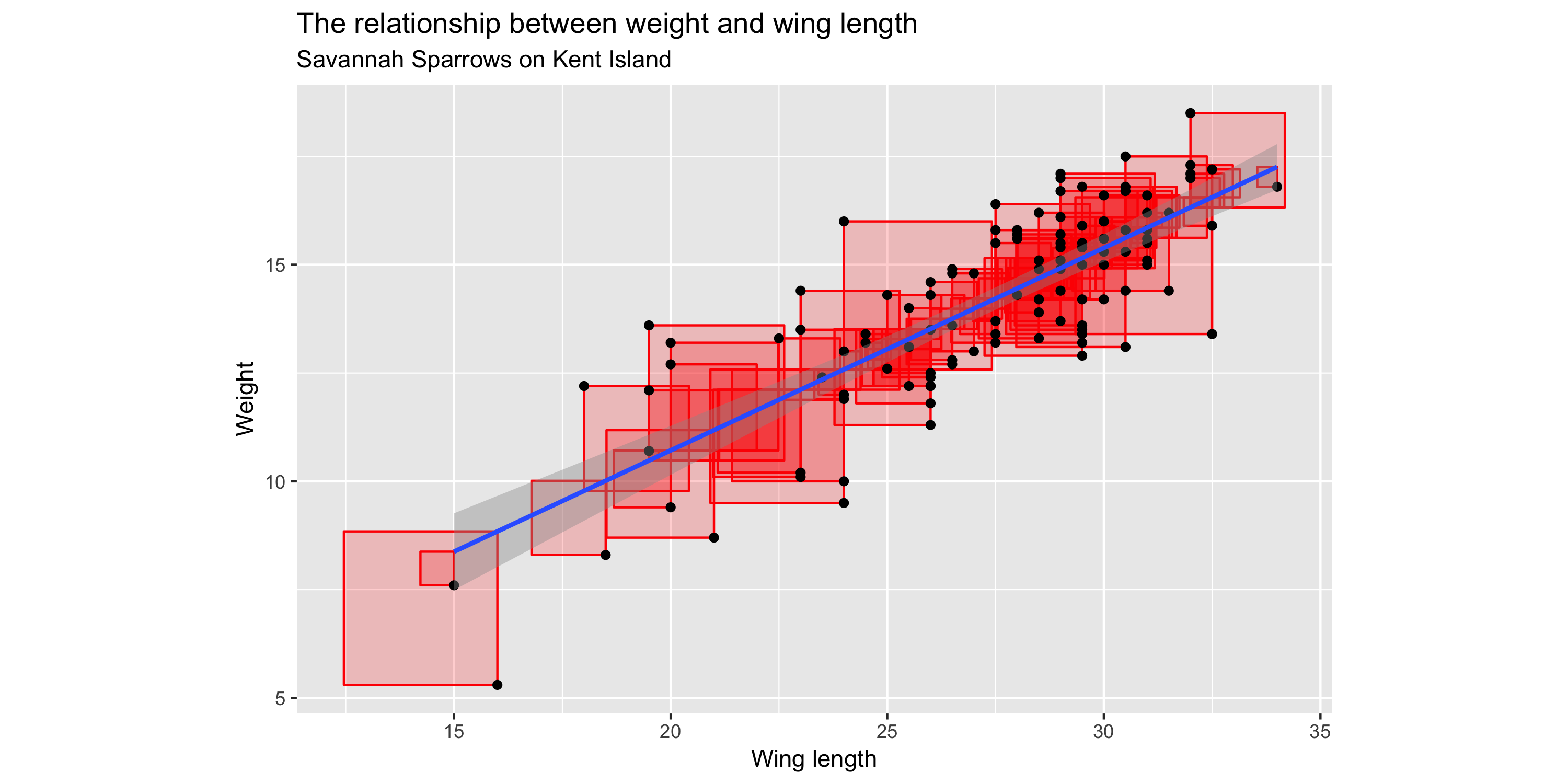"Residuals"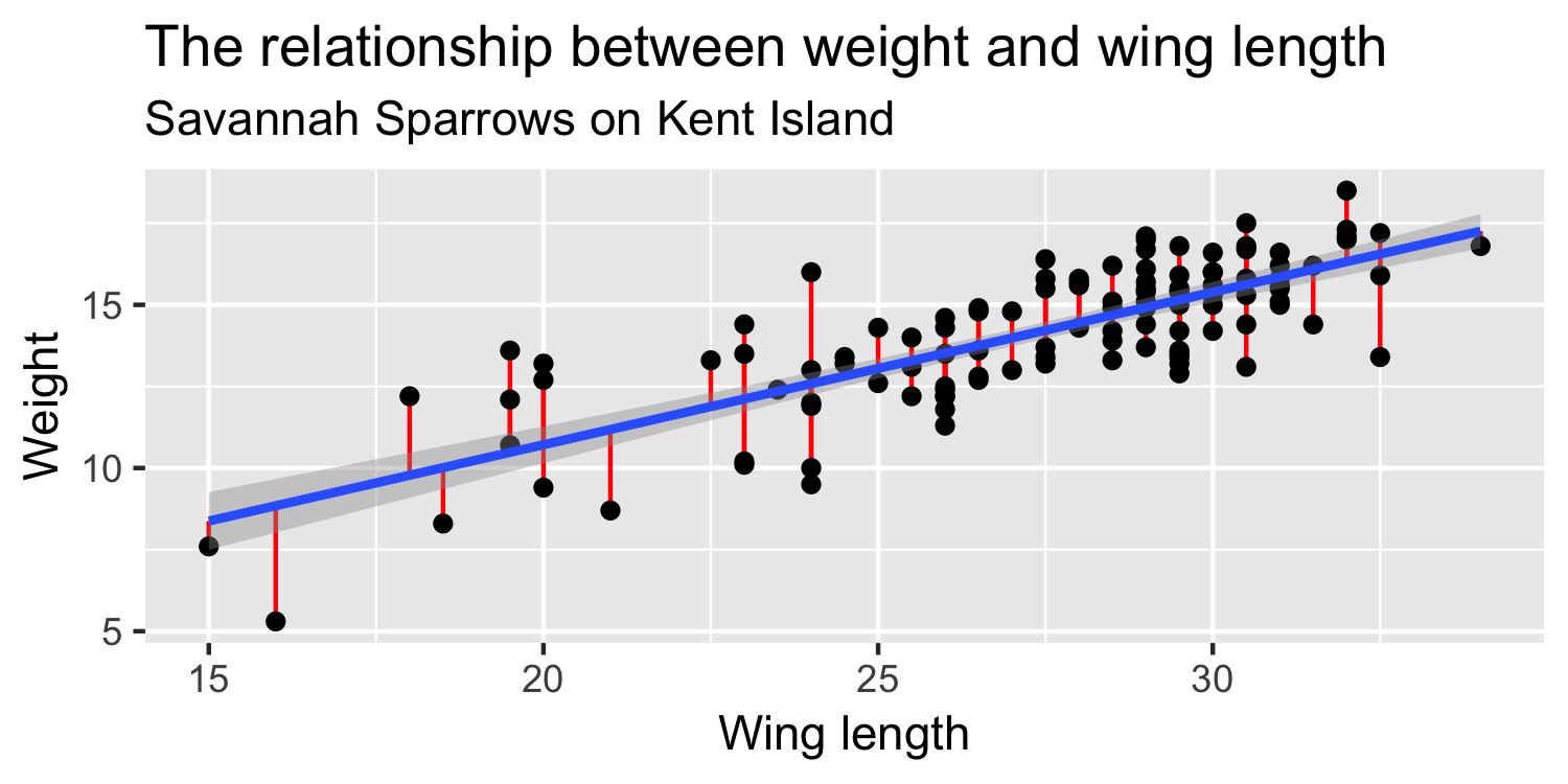

Definitions

• residual $\left(e\right)$
• squared residual $\left(e^2\right)$
• sum of squared residual (SSE)
• standard deviation of the errors $\left({\sigma }_{ϵ}\right)$
• n

Definitions

• residual $\left(e\right)$: observed $y$ - predicted $y$ $\to$ $y-\hat{y}$
• squared residual $\left(e^2\right)$: $(y-\hat{y}{)}^2$
• sum of squared residual (SSE): $\sum (y-\hat{y}{)}^2$
• standard deviation of the errors $\left({\sigma }_{ϵ}\right)$: estimated by ${\hat{\sigma }}_{ϵ}=\sqrt{\frac{SSE}{n-2}}$ (regression standard error)
• n: sample size

☝️ Note about notation

• $\sum (y-\hat{y}{)}^2$
• ${\sum }_{i=1}^n(y_i-{\hat{y}}_i{)}^2$

☝️ Note about notation

☝️ Note about notation

☝️ Note about notation

Calculate the residual

y_hat <- lm(Weight ~ WingLength, data = Sparrows) %>%
  predict() 
Sparrows %>%
  mutate(y_hat = y_hat,
         residual = Weight - y_hat) %>%
  select(Weight, y_hat, residual) %>%
  slice(1:5)

##   Weight    y_hat    residual
## 1   14.9 14.92020 -0.02020496
## 2   15.0 15.85501 -0.85501292
## 3   14.3 13.05059  1.24941095
## 4   17.0 14.92020  2.07979504
## 5   16.0 15.38761  0.61239106

Calculate the squared residuals

y_hat <- lm(Weight ~ WingLength, data = Sparrows) %>%
  predict() 
Sparrows %>%
  mutate(y_hat = y_hat,
         residual = Weight - y_hat,
         residual_2 = residual^2) %>%
  select(Weight, y_hat, residual, residual_2) %>%
  slice(1:5)

##   Weight    y_hat    residual   residual_2
## 1   14.9 14.92020 -0.02020496 0.0004082405
## 2   15.0 15.85501 -0.85501292 0.7310470869
## 3   14.3 13.05059  1.24941095 1.5610277150
## 4   17.0 14.92020  2.07979504 4.3255474012
## 5   16.0 15.38761  0.61239106 0.3750228116

Calculate the SSE

y_hat <- lm(Weight ~ WingLength, data = Sparrows) %>%
  predict() 
Sparrows %>%
  mutate(y_hat = y_hat,
         residual = Weight - y_hat,
         residual_2 = residual^2) %>% 
  summarise(sse = sum(residual_2))

##        sse
## 1 223.3107

Calculate the regression standard error

y_hat <- lm(Weight ~ WingLength, data = Sparrows) %>%
  predict() 
Sparrows %>%
  mutate(y_hat = y_hat,
         residual = Weight - y_hat,
         residual_2 = residual^2) %>% 
  summarise(sse = sum(residual_2),
            n = n(),
            rse = sqrt(sse / (n - 2)))

##        sse   n      rse
## 1 223.3107 116 1.399595

Calculate the regression standard error

##        sse   n      rse
## 1 223.3107 116 1.399595

lm(Weight ~ WingLength, data = Sparrows) %>%
  summary()

## 
## Call:
## lm(formula = Weight ~ WingLength, data = Sparrows)
## 
## Residuals:
##     Min      1Q  Median      3Q     Max 
## -3.5440 -0.9935  0.0809  1.0559  3.4168 
## 
## Coefficients:
##             Estimate Std. Error t value Pr(>|t|)
## (Intercept)  1.36549    0.95731   1.426    0.156
## WingLength   0.46740    0.03472  13.463   <2e-16
## 
## Residual standard error: 1.4 on 114 degrees of freedom
## Multiple R-squared:  0.6139,    Adjusted R-squared:  0.6105 
## F-statistic: 181.3 on 1 and 114 DF,  p-value: < 2.2e-16

Porsche Price

• Go to RStudio Cloud and open Porsche Price
• For each question you work on, set the eval chunk option to TRUE and knit

Linearity

The overall relationship between the variables has a linear pattern. The average values of the response $y$ for each value of $x$ fall on a common straight line.

Zero Mean

The error distribution is centered at zero. This means that the points are scattered at random above and below the line. (Note: By using least squares regression, we force the residual mean to be zero. Other techniques would not necessarily satisfy this condition.)

Constant Variance

The variability in the errors is the same for all values of the predictor variable. This means that the spread of points around the line remains fairly constant.

Independence

The errors are assumed to be independent from one another. Thus, one point falling above or below the line has no influence on the location of another point. When we are interested in using the model to make formal inferences (conducting hypothesis tests or providing confidence intervals), additional assumptions are needed.

Random

The data are obtained using a random process. Most commonly, this arises either from random sampling from a population of interest or from the use of randomization in a statistical experiment.

Normality

In order to use standard distributions for confidence intervals and hypothesis tests, we often need to assume that the random errors follow a normal distribution.

Summarise conditions

For a quantitative response variable $y$ and a single quantitative explanatory variable $x$, the simple linear regression model is

$y={\beta }_0+{\beta }_{1}x+ϵ$

where $ϵ$ follows a normal distribution, that is, $ϵ\sim N(0,{\sigma }_{ϵ})$, and the errors are independent from one another.

broom

library(tidyverse)

library(broom)

## Warning: package 'broom' was built under R version 3.5.2

Porsche Price

• Go to RStudio Cloud and open Porsche Price